Free ebook

HOW TO BUILD AI-driven object detection software

A step-by-step guide for CTOs and tech leaders

AI’s been on our minds for a long time

But until recently, it’s been reserved for huge enterprises and complex projects. See what it takes to build your own AI-powered object detection software using deep learning and synthetic data, for things like:

Image content matching

Targeted advertising

Social media monitoring

What’s inside?

1 Establish the metrics

2 Data collection

3 Bulding a data-set (and enhancing it with synthetic data)

4 Training the model and testing performance

5 Deploying the model to production

6 Monitoring and optimizing performance

format_quote

Establish the metrics

Setting the project scope

Defining the scope of any data science project is a crucial first step — more so than for any other project type.

And every data science project must start with the project or business need: the outcome we’re ultimately seeking to serve. Once we’ve defined our need, it’s time to validate any and every assumption — either by talking to customers, or through discussing them with relevant businesses.

A product owner should lead these conversations. It’s here where we start to develop an idea of how the future feature set-will evolve. And while it is rare, at this stage, for any stakeholder to have a full vision of what the product will ultimately look like; it should be possible to describe the product in terms of ‘the problem(s) our business is currently facing.’

It’s important that product owners and data scientists collaborate throughout the problem definition process as a close working relationship will allow the data scientists to elaborate on the category of project the product fits.

Working together allows them to answer questions like:

‘Is it a ‘classification’ problem or ‘segmentation’ problem?
What kind of data exists to power possible solutions?
Can we access this data and if yes, how much data is there?
What is the quality of the data?

Answering these questions early on is a crucial first step in understanding the problem. Moreover, once we know the answers, we can move onto defining the exact scope during the research phase.

Here, we explore existing open source libraries, state-of-the-art solutions, and scientific papers focused on the subject matter with the aim of validating the project scope.

With the scope understood, now onto the crucial second stage of setting the KPIs of the project itself. When setting KPIs, make sure to settle on metrics that are:

Accepted by the business
Accepted by the tech team
Clear and easily measured

As if we fail on 1, 2, or 3, we will struggle to communicate progress to stakeholders, determine when the project is actually over, or say with any confidence if the product was, indeed, successful.

With the above in mind, let’s move onto how we define our KPIs.

Defining the KPIs

KPIs are crucial to any project. They are our North Star as we sail the high-seas of the unknown.

An example of a clear KPI could be something like “detecting logos on an image with an f1 score >0.98.”

That said, projects often have too intangible an output (e.g., if we’re measuring the ‘perceived customer experience’) to assign such a concrete metric — or they deal with complex human behaviors that are near- impossible to measure in numbers.

In these instances, we suggest using less specific KPIs, like “most of the pictures that have had their background automatically removed still preserve their overall quality and are acceptable to users.”

Such a KPI offers enough general direction to start development. However, when it comes to setting acceptance criteria, it is inadequate: extra details are needed.

To make the example concrete, let’s imagine we run a travel website. And we want to check if our users have uploaded photos of winter or summer.

In reality, this is a very typical computer vision request.

For this type of project, the product owner first needs to identify the kind of information they need to extract, alongside the level of precision needed (the success KPI) in order to satisfy the “winter vs. summer” image recognition requirement.

Depending on the product owner’s specifications, the data science team can then train an AI algorithm to execute a selection of tasks to retrieve the information requested from the images.

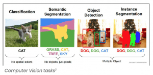
To understand the problem in more detail, let’s first walk through the different image recognition technologies available. And elaborate on the distinct problems each one is designed to solve. We can then take a closer look at what outputs indicate good project performance.

First up, let’s review the available technologies — you can see each one in action by looking at the images on the next page:

Classification
Detection
Segmentation

A. Image Classification

Image classification is a core task in Computer Vision. Its primary objective is to classify an object in the image based on predefined classes.

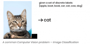
The problem may appear trivial to the human eye. However, for a computer vision system, it presents many complex challenges.

Just think of all the viewpoint variation, background clutter, illumination, deformation, occlusion, and intraclass variation that could confuse a non-human viewer (see examples below).

And remember: a computer only sees images as a basic number grid, ranging between [0, 255], and usually in three channels — with each channel representing a color: red, green, or blue.

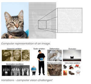
There’s no obvious way to hard-code a standard computer program to recognize a cat (or any other object in a picture, for that matter).

As such, until Deep Learning started to be applicable to real-world Computer Vision problems in the early 2010s, any Computer Vision task required significant expertise to complete.

Convolutional Neural Networks (CNN) emerged from the study of the brain’s visual cortex, which developers have used in image recognition since the 1980s.

In more recent times — thanks to the increase in computational power, coupled with the growing volume of data that’s available to train an algorithm — CNNs have managed to achieve superhuman performance on several complex visual tasks.

And with Deep Learning-based solutions dominating the ImageNet Challenge from 2012 onwards, this illustrates the power of Convolutional Neural Networks.

ROUND-UP: IMAGE CLASSIFICATION

Problem Definition

Image Classification refers to the task of assigning a label to an image from a fixed set of categories. It is one of the core problems that Computer Vision aims to solve and, despite its apparent simplicity, it has a large variety of practical applications.

Moreover, many other seemingly separate Computer Vision tasks (such as object detection or segmentation) can be reduced to Image Classification.

Suggested Approach

As there’s no obvious solution for writing an algorithm to identify, say, the shape of a cat in an image, it can be more effective to try to specify what the categories look like in the codebase itself.

Taking this approach, we’re going to provide the computer with many examples of each category. Then, develop a machine learning algorithm that looks at these examples and learns about the visual appearance of each class in the code.

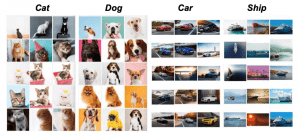
This process is known as the data-driven approach (given it relies on accumulating a training data-set of labelled images). Below is an example of what such a training data-set might look like.

Classification KPIs

We can assess the accuracy of an image classifier by asking it to assign labels to a new set of images that it has never seen before. We can then compare the correct tags for these images with the ones assigned by the classifier and draw the following conclusions:

If the predictions match the correct answers (which we call the ground truth), we can infer that the classifier is working to a high degree of accuracy;
If the predictions do not match the correct answer, the error rate (the ratio of wrong predictions to all predictions) is too high.

It is common to report two error rates: ‘top-1’ and ‘top-5.’

Top-5 refers to the fraction of test images for which the correct label is not among the five labels considered most probable by the model. We report a top-5 error rate as real-world objects:

Can be multiple things

Can be one thing or another

Or can be easily confused

Equally, there could be a hierarchy (for example, a fireman is a person and a rose is a flower). However, as real-world relationships are complicated — and sometimes relative — in most cases, these are considered as separate, unrelated classes.

Finally, if we gave a classification problem to several people, we would likely get multiple different answers. Therefore, we need to check if a class deemed ‘most suitable’ to an image is, in fact, among the classes that the automated solution considers ‘most probable.’

Multilabel classification

Up until now, the example images have contained a single object (more or less). Obviously, this will not always be the case.

What if an image contains a cat as well as a dog, yet our model has to predict a single label?

It’s hard to define the correct outcome: cats are often overrepresented in datasets (they are the internet’s favorite image, after all!), but a dog may be bigger in the picture.

In this case, we could use a technique called ‘multilabel classification,’ which lets us predict multiple labels for a single image.

In theory, the network architecture for such a problem wouldn’t be all that different from before. Networks usually end up predicting probabilities for each class, either way.

However, as greater attention is needed in terms of the scale of the objects — as they don’t fill the frame and because a network should be trained on a different dataset — in practice, the architectures are different.

Therefore, instead of accuracy, we use the F1 score metric, which takes into account:

Precision — as a fraction of relevance among the retrieved images; and,

Recall — as a fraction of relevance among the retrieved images.

Precision scores ‘1’ if all elements deemed class A are genuinely from this class. If not, precision scores lower.

Recall scores ‘1’ if all of the elements from class A are labeled as such — any missed element means recall scores lower.

Given the above, the F1 score is a harmonic balance of precision and recall.

If we simply need to classify several objects in an image, then object detection is the better bet (see the next section). Saying that, multilabel classification enables us to do something more complex: to label abstract concepts.

An image may depict a ‘scene from a cafeteria’ or an ‘activity like running.’ A picture may show ‘nature’ or simply, ‘a forest.’ These are not objects in the way a ball, a cat, a building or a ship are. And often, they cannot be pinpointed on an image.

Still, they are tangible and recognizable concepts and they can be labelled.

B. Object Detection

There are two distinct object detection tasks. They use either ‘bounding box’ or ‘object segmentation’ (the latter is also known as ‘instance segmentation’).

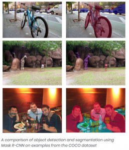
Object Detection is relevant for anyone looking to identify a specific object within a selection of images.

The output can include a rectangle on the image — also called a ‘bounding box’ — that pinpoints the object’s location; or, a mask can show which part of an image the object occupies.

Object Detection can also involve a computer program that identifies the position of all objects (e.g. pedestrians) in a frame, in which case it could count how many people there are in a crowd.

We could then use this information to plan the capacity for how many passengers a train or subway carriage can transport. Equally, we could apply the technology to the context of video surveillance and identify when someone enters a room — or when a crowd exceeds a certain number of people.

ROUND-UP: OBJECT DETECTION

Problem Definition

Object Detection refers to the task of classifying and locating multiple objects in a range of different images.

Suggested Approach

Until recently, a common approach to Object Detection was using a CNN trained in classifying and locating a single object, then sliding the CNN across the image.

Users would then continue to slide the CNN over the whole image and, given objects can vary in size, also slide the CNN across regions of different sizes as well.

This simple approach to Object Detection works quite well. However, as it requires running the CNN many times, it is a slow process. Fortunately, there’s a much faster way of sliding a CNN across an image: that is, by using a Fully Convolutional Network (FCN).

The FCN approach is much more efficient than the CNN approach given the network only looks at an image once (‘You Only Look Once’ — YOLO — is, in fact, the name of a very popular object detection architecture).

Other popular Object Detection models include Single Shot Detection (SSD) and Faster-RCNN.

But the best detection system to use will depend on many factors, including but not limited to speed, accuracy, the availability of pre-trained models, training time, and complexity.

Detection KPIs

A common KPI used in Object Detection is the ‘mean Average Precision’ (mAP).

To get a fair idea of the model’s performance, we can use mAP to compute the maximum precision we can get with at least 0% recall (then, 10% recall, 20%, and so on, up to 100%).

We can then calculate the mean of the results, known as the ‘Average Precision’ (AP) metric. And when there are more than two classes, we can compute the AP for each class — then, calculate the mean AP (mAP).

Common Objects in Context (COCO) describes twelve detection evaluation metrics:

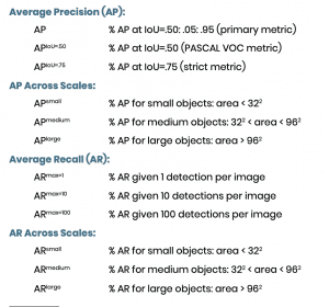
The use of a more specific metric than AP may be beneficial if our problem has a specific characteristic. For example, if the objects in the image are small, we may use AP-small and AR-small.

C. Image Segmentation

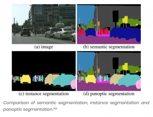
If you need to classify each and every pixel of an image, then you should use Image Segmentation (also known as ‘Semantic Segmentation’ — illustration below).

Image Segmentation maps each pixel to a class.

It does not care how many objects are there and, if there are overlap-ping objects of the same class, they will be labelled as a single ‘blob.’

Due to its nature, image segmentation often relies on higher-level concepts like grass, road, sky, water, ground: concepts that are not finite objects in terms of a picture.

This is one of the reasons why image segmentation has become so widely used in healthcare in general, and in cancer detection in particular.

We could use image detection to label types of cells or types of tissue — like epithelial, connective, muscular, and nervous — or, simply ‘normal’ and ‘abnormal.’

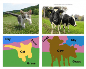
Image segmentation may be seen as a trade-off when compared to instance segmentation. But it should really be thought of more like a specialized tool.

Detecting and segmenting each-and-every cell in a medical image would not be useful in most cases. Just like when working with objects of continuous nature — like a splash of paint or a group of cancerous cells — instance segmentation could cause confusion.

In such cases, ‘semantic segmentation’ can deal with the fluid borders; even though these still require a sharp result.

At this stage, it’s worth noting the emergence of a new field: ‘panoptic segmentation.’ Panoptic segmentation aims to unify semantic segmentation with instance segmentation.

It offers a complete segmentation in the same way image segmentation does, but keeps instances of the same class, separate.

ROUND-UP: IMAGE SEGMENTATION

Problem Definition

In image segmentation, each pixel is classified according to the class of object to which it belongs (e.g., road, car, pedestrian, building, etc.).

It’s important to note that different objects of the same class are not distinguished: for example, all the bicycles in a segmented image may end up as one big clump of pixels tagged ‘bicycle’.

The main difficulty of image segmentation is that when an image goes through a standard CNN, it gradually loses its spatial resolution (due to the layers with strides greater than 1).

When each convolutional filter is applied, it slides over the image and each convolution result is a single pixel of the next layer’s image.

If the stride is 1: each time a filter moves, a single pixel and output resolution is the same as the input (with appropriate padding). Oftentimes, however, the stride is greater than 1.

This is beneficial to performance in terms of both speed and accuracy, as it allows us to consider long-distance relationships cheaply. However, astride of X also reduces the size of the image by a factor of ‘X.’

As such, a regular CNN may end up ‘knowing’ that there’s a person in the image “somewhere in the bottom left” — but it cannot be more precise than that.

Suggested Approach

As with object detection, there are several possible approaches to tackling image segmentation, with some more complex than others.

A relatively simple solution was proposed in a 2015 paper by Jonathan Long et al. The paper suggests taking a pre-trained CNN, which you can turn into an FCN.

The CNN applies multiple convolutions with various strides to the input image, which results in the last layer of outputs featuring maps that are way smaller than an input image (e.g. up to 32x smaller).

In practice, this process delivers too coarse a result.

Therefore, the paper proposed adding a single up-sampling layer to multiply the resolution by 32 (there are several solutions for up-sampling, including bilinear interpolation, but they only work reasonably well up to x4 or x8 — not x32).

Therefore, as an alternative approach, the researchers used a transposed convolutional layer, which is the equivalent of interleaving an image with empty rows and columns (full of zeros), then performing a regular convolution.

Some people prefer to think of the adopted approach as a regular convolutional layer that uses fractional strides (e.g., 1/2).

The transposed convolutional layer can be initialized to perform something close to linear interpolation. But given it is a trainable layer, it will learn to perform better, the more it trains.

Segmentation KPIs

Image segmentation is all about predicting the class of each pixel in an image. There are two leading KPIs used to measure its efficacy. And the first is Intersection over Union (IoU) — also referred to as the Jaccard Index.

Intersection over Union

IoU quantifies the percentage overlap between the target mask and our prediction output.

This metric is closely related to the Dice coefficient, which is often used as a loss function during training. Simply put, the IoU metric measures the number of pixels-in-common between the target and prediction masks, divided by the total number of pixels present across both masks.

As a visual example, let’s suppose we’re tasked with calculating the IoU score of the following prediction, given the ground truth labelled mask.

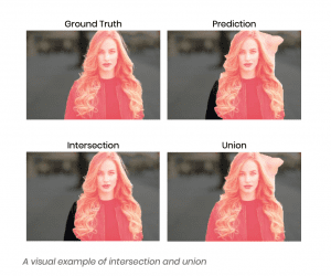
The IoU score is calculated for each class separately and then averaged over all classes to provide a global, mean IoU score of our semantic segmentation prediction.

Pixel Accuracy

The second metric for evaluating image segmentation is to report the percentage of pixels in an image that were classified correctly, known as Pixel Accuracy.

This KPI is typically reported separately per class, as well as globally across all classes, and when considering the per-class pixel accuracy, we’re essentially evaluating a binary mask:

A true positive represents a pixel that is correctly predicted to be- long to the given class (according to the target mask);
A true negative represents a pixel that is correctly identified as not belonging to the given class.

This metric can sometimes provide misleading results.

Particularly, when the class representation is small within the image — as the measure will be biased towards how well we identified the negative case (ie. where the class was not present).

Now we’ve covered KPIs, let’s move onto section 2: data collection.

Data collection

Once we have defined the problem, the next step is to clarify the type of data we need to build our image detection system. This is the data we will use to train our model.

Still, one question remains:

— “What type of training data do we need to collect?”

Ultimately, the answer depends on the specifics of the project we’re working on. However, there are several key factors that every product owner must consider, no matter the focus of their work.

These are:

Data accuracy
Data diversity
Data quantity
Data quality

Let’s look at each factor in detail to help you understand precisely what we mean.

Data Accuracy

Imagine we’re trying to build a tool that ‘removes the background from pictures with people.’ In this instance, there’s no point in using photo- graphs without people in them, as they won’t help to train our model.

Put another way; data accuracy is about finding pictures that serve our problem, specifically.

So, while we can easily find extensive photo databases online: the challenge rests in finding a data-set that encapsulates the problem we’re trying to solve.

Data Diversity

Once we’ve collated a representative data-set, the next hurdle is to ensure our training data is sufficiently diverse across all the aspects we’d like to extract.

For instance, if we’re looking to solve the problem of ‘detecting all cars in a photo’ — we need as many images as possible, showing as many different models of vehicles as possible.

Moreover, we need various colors, angles, and settings to get a high-quality result (there may be many red Ferraris driving around Miami Beach, but not all of them are).

Equally, if we’re merely interested in ‘identifying the cars on a city street,’ we won’t need pictures of F1 vehicles in our data-set.

Data Quantity

The rule of thumb says, “More is better’ — but everything depends on the problem we’re trying to solve.

Sometimes, we’ll need tens of millions of images to train our algorithm. Other times, a few hundred photos will suffice (maybe less); it all depends on the task, the anticipated performance of the model, and the use case(s) at hand.

The larger the diversity and the more difficult the problem, the larger the dataset has to be.

For instance, if we’re hoping to detect a person’s wrist, and the setting is a purpose-built lightbox (simply put, a tent that allows photography to happen in an appropriately lit environment, without shadows), then it’s a relatively simple task.

In contrast, if we want to detect a person’s wrist in the natural world, where lighting conditions and shadows vary greatly, the task isn’t so straightforward.

If we wanted to detect a hand in place of a wrist, the same context applies.

But while you may think the difficulty is the same, that’s not the case at all. In fact, even though the apparent problem is similar, it’s much easier to detect a hand than a wrist — as a hand has many more distinctive features (fingers, for a start!).

If you need novel ways to increase your data-set, we will explore your options in ‘Section 3: Building Your Data-set’ but first, let’s look at data quality.

Data Quality

Finally, what role does data quality play in machine learning?

Is there a measure that dictates which pictures we should (or shouldn’t) use? Typically, it’s safe to assume that if a person can perform a task on any given image, then the quality is OK for the machine as well.

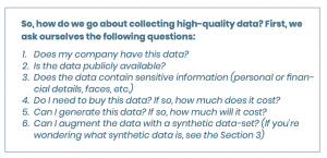
Depending on the answers, it could be quick and cheap to collect the data we need. On the other hand, we may need to allocate resources and find the budget to carry out the data collection exercise.

If the latter is the case, we may even have to delay building the model to first create a system to collect the information we need, but remember: that’s par for the course as a comprehensive data-set sits at the core of every machine learning project.

Bulding a data-set (and enhancing it with synthetic data)

How to Build a Data-set

Once we have our initial data-set, it’s possible we haven’t covered all the necessary features or edge-cases. Maybe we lack sufficient data to build an accurate model — but what can we do?

Well, the answer is simpler than you might think. We can augment our data-set with synthetic data.

However, before we get into discussions around how we go about generating synthetic data, let’s first focus on what a ‘proper data-set’ really is.

To train a model to detect a specific image, we first need to tell the algorithm what our pictures contain via a process known as data labeling: data labeling tells our algorithm to associate each image in a data-set with a particular label.

Depending on the problem we’re trying to solve, we can use different labels based on the tasks we want the algorithm to perform (segmentation, detection, or classification).

At this point, you may have to face up to the fact that annotating is time-consuming.

In most cases, it’s a manual process that has to be done by humans. Perhaps, it forms part of a daily workload (say, radiologists annotating cancerous cells). However, oftentimes, the work is an extra task which is not required for humans to solve the problem, but is for a machine to learn it.

Thankfully, annotation training images can normally be outsourced to specialized agencies.

That said, if you’re processing sensitive data — or annotating is a specialty of yours — it may be best to keep the exercise in-house. Otherwise, feel free to delegate the task to a third-party (there are agencies that specialize in data annotation).

Bear in mind that it may be important for the same picture to be annotated by several people (perhaps, to account for varying perspectives): if so, make sure the requirement is clear so that you maximize the quality of the data.

If building an in-house annotation team, consider using tools like Label- Me; or find the option that best-suits your project needs — while accounting for ease of setup, use, and the ultimate project goal.

DLABS PRO TIP

How do you find the best annotation service for your project? We’ve collected this handy checklist to help you out:

1. Weigh the pros and cons of available solutions and decide which one works best for you:

A. Hire own annotators

Pros: secure, fast (once hired), less Quality Control (QC) needed
Cons: Expensive, slow to scale, admin overhead

B. Crowdsource (Mechanical Turk)

Pros: cheaper, more scalable
Cons: not secure, significant QC effort required

C. Full-service data labelling companies

As data labelling requires a separate software stack, temporary labor, and quality assurance — it often makes sense to outsource this entire task.

In all the above solutions, training the annotators is crucial and quality assurance is key. If you decide to use a third-party service, make sure to:

Dedicate several days to finding the best provider
Shortlist several candidates and ask for work and data samples
Label ‘gold standard data’ yourself — in other words, create a database of representative or critical images that you label yourself and from which the service company can learn how to label the remaining images correctly
Agree to a gold standard, and evaluate each proposal based on the cost of the service

Ultimately, there are two schools of thought when it comes to data collection: either you need more data for the best outcome — or, you need better quality data to achieve the best results.

We can assess the above by looking at an example from a different, but well-known domain: Netflix recommendations.

Netflix offered a prize of $1m to anyone who could design a movie re- commendations algorithm that performed better than the one developed by Netflix itself.

Some practitioners, including Anand Rajaraman, claimed that ‘more data usually beats better algorithms.’

However, to counter that point, Pilaszy and Tikk later wrote a paper concluding that as few as ten ratings of a new movie are more valuable than all the available meta-data for predicting user ratings.

In their case, they claimed quality outperformed volume.

Switching back to computer vision, the ability to transfer learning and pre-train a model significantly lowers the need to have ‘lots of data’ at your disposal.

Moreover, resources like Imagenet also contain millions of training images across different categories, with models pre-trained on all of them.

Therefore, we can use this information provided our domain is somewhat similar to Imagenet (it doesn’t have to be identical), and we won’t need to source millions of original images to get good results — all we need to do is start with a pre-trained model and fine-tune the weights to our specific dataset.

It’s up to you to decide which camp you fall into, but sourcing lots of high-quality data is always the safest bet.

Enhancing A Data-set With Synthetic Data

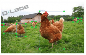
In recent years, people in all walks of life have used deep learning algorithms to solve problems associated with object detection.

In a business context, enterprises have saved significant time and money using the approach to automate key workflows — for example, by detecting faulty products on a production line using bespoke quality assurance systems. That said, it takes a vast set of appropriately tagged data to build such a detector model or service.

Typically, the tagging also requires a specific label that indicates the position of an object category via a set of coordinates — called a bounding box — detailing precisely where the object sits in the image.

Here, a conflict arises…

Most companies want to develop and deploy their AI services ‘as fast as possible’ and preferably ‘with minimal data preparation’ — whereas the collection of data, coupled with the labeling of target objects, is a time-consuming, burdensome, and expensive process.

— So, what can we do to ease the workload?

Data labeling approaches

The following table presents the spectrum of approaches to data labeling. It highlights the primary factors that influence the method of choice.

More often than not, however, the chosen route comes down to little more than available financial and human resources.

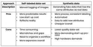
Weighing up the options

If we have data without target bounding boxes and labels, we must annotate the images: a process we can either manage internally or out-source to a third-party — say, to Amazon’s Mechanical Turk or Yandex Toloka…

… Or, we can generate synthetic data.

The benefit of generating synthetic data is that the objects we are ultimately trying to detect have been added to the images as part of the data generation process.

As such, we already know their labels and bounding boxes, which removes a step from the annotation process.

This fact alone can substantially speed up the process compared to manually marking images, which makes the approach very attractive to some.

However, it’s vital to remember the pros and cons of real versus synthetic images as these can dictate the final utility of the data and determine which of the methods is best suited to your project.

So, what’s the takeaway?

Never just assume that one way is better than the other: verify your choice under real-world operating conditions.

Case study: Creating Synthetic Data For Logo Detection

For some established brands (especially those that have been around for a few years), there may be thousands of existing photos available online.

For the rest of us, synthetic data may be our only option.

The same applies to recommendation engines (like with Netflix) where the algorithm’s task is to recommend the next item to watch based on a user’s past purchases, choices and preferences.

In this case, we use the term ‘cold start.’

In this section, let’s look at an experimental study of the described approach, using logo detection as an example of how to create synthetic data.

In DLabs’ case, we created synthetic images by applying transformations to photos that already contained logos, then blended them with background images, using background depth information and additional augmentations — we then tested the algorithm’s accuracy using real images.

There are several other approaches you can use to achieve a similar result, one of which is known as SynthLogo.

SynthLogo is based on the synthesis pipeline used in SynthText [M. Jaderberg, K. Simonyan, A. Vedaldi, and A. Zisserman, “Reading text in the wild with convolutional neural networks,” International Journal of Computer Vision, vol. 116, no. 1, pp. 1–20, January 2016].

SynthText blends rendered text into background images, with the image synthesis process consisting of five steps:

Download background image
Download logo
Segment information in background image
Estimate the depth of background image
Blend logo images using augmentation
Generating an image pipeline

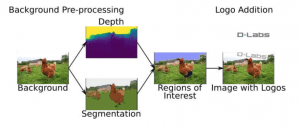
SynthLogo: In-depth Process

To kickstart the SynthLogo process, we first needed to download a background image and logo file to use when training our logo detection models.*

*Note: You could use any resource for this, Google Search worked fine for us. We just had to double-check that images didn’t already contain a logo from within our data-set and, given brands can have multiple versions of a logo, we also had to check that no variant was present… while each file had to be in .PNG format with alpha channel.*

We then obtained depth information via a Convolutional Neural Network (as described in [F. Liu, C. Shen, and G. Lin, “Deep convolutional neural fields for depth estimation from a single image,” Proceedings of the IEEE Conference of Computer Vision and Pattern Recognition, pp. 5162– 5170, June 2015, Boston, MA.]).

We segmented the background images by detecting the contours of the elements that formed the image (as described in [C. F. P. Arbelaez, M. Maire and J. Malik, “Contour detection and hierarchical image segmentation,” IEEE Transactions on Pattern Analysis and Machine Intelligence, vol. 33, pp. 898–916, May 2011]) — and we discarded small segments, or segments with extreme aspect ratios.

Next, we selected a segment of a background image from all the suggested segments. And using the depth information, we transformed the logo geometrically so that it matched the estimated surface orientation.

For this step, we used the Random Sample Consensus (RANSAC) method [M. A. Fischler and R. C. Bolles, “Random sample consensus: A paradigm for model fitting with applications to image analysis and automated cartography,” Communications of the Association for Computing Machinery, vol. 24, no. 6, pp. 381–395, June 1981.].

Then, before blending, we changed the logo image using a transformation step (e.g., rotation, color jittering with some probabilities).

Finally, we blended the logo into the background, with the blending pro- cess combining the pixels of the background image with the pixels of the transformed logo (note: we played with alpha layer here as well).

Results

Using this process, we were able to generate roughly 50,000 images and build a model that performs to an acceptable level of accuracy.

If we assume that labelling a single image could take a worker 30 seconds, then it would take over 52 human days to achieve the same results via a manual process.

When looked at in light of the below, you can see how the synthetic approach can offer significant cost savings:

Labelling 50,000 images (assuming the price for each image is $0.05) on a crowdsourcing platform would cost $2,500
If you were to use a synthetic data set, you would only pay for an instance on OVH with 30GB RAM — in the context of the process outlined above, our cost was less than $10

Moreover, our model could now automatically generate any number of synthetic labelled logo images in a realistic context with minimal supervision.

This data-set is then appropriate for training logo detection CNN networks (such as region-based convolutional neural networks) and obtained promising results when tested on FlickrLogo dataset.

Unfortunately, this method would not work if we were trying to detect objects that were not independent from their background but were, instead, background alterations and anomalies — or if they had complex interactions with the background.

For example, our method would not work to detect ‘changes in an X-ray image.’

In such a context, synthetic data generation would be at least as complex — not to mention as expensive — as the original detection challenge.

Training the model and testing performance

There are many applications for image analysis. Let’s maintain focus on the simplest task, that of classification.

As our classifier, we will use neural networks: a general-purpose tool that can be used for a wide range of applications with high precision. If such networks have several hidden layers (other than input and output layers), we will call them ‘deep.’

Inspiration

The construction of these networks was originally inspired by natural biological processes.

In the 1960s, a famous experiment with cats’ primary visual cortex was conducted, which confirmed that each of us has neurons that are responsible for some specific characteristics (such as those that capture movement, different colors, horizontal or vertical lines, etc.).

These same neurons that are responsible for vision are not „general” — every single one has its own unique task, which, in total, make up the larger characteristics of vision.

As you can see: neural networks are inspired by how the brain (be it human or feline) functions.

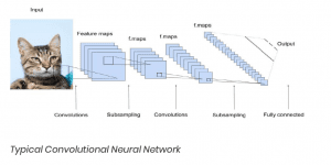
As spatial relations are crucial in image processing, we use convolutional layers. These layers are also inspired by biology: a neuron can re- cognize a complex feature by using the output of neighboring neurons detecting simpler ones.

In artificial neural networks: after the many convolutional layers, we find a dense — or ‘fully connected’ — layer, which depends on the network and how sparse or dense it is.

Diving into the detail of the architecture of a convolutional network: it consists of several components.

In the initial layers, there’s a split into color channels
Each channel is then subjected to a linear operator
The result is acted on by another layer — a max-pooling operator — whose function is to detect the fragments of the image in which there are interesting features

The output of this admittedly complicated initial data processing is given as an input to a fully-connected neural network (a multi-layer perceptron — or MLP).

In intermediate layers, there are convolutional layers of further rows and the activation function is not sigmoid (a sigmoid function is a type of activation function that limits the output to a range between 0 and 1), but e.g. ReLU (rectified linear unit), another type of activation function.

The advantages of using ReLU are computational simplicity and solving the vanishing gradient problem.

The output from such a network can be a vector, which can be interpreted as features, tags, descriptions — or whatever is required.

Another popular approach is the use of recursive networks, which retrieve the image at the input.

Over several iterations, the network can then make various modifications — for example, improving sharpness, or returning other images from its memory that are very similar to the original input image.

The brain has relatively few layers compared to artificial networks. But the layers of the brain are interconnected by vast numbers of neurons, which makes it such an effective learning machine.

Still, artificial networks can learn.

They can learn to capture and describe objects, or to process them into some form or other. Today, there are countless ready-made network architectures available on the Internet (including the You Only Look Once architecture referenced earlier in this paper).

And once they’ve processed an image and labelled the interesting objects, they can describe the image in almost real-time.

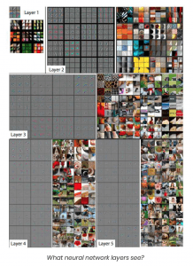
The figure above shows the visualization of features of a fully trained model in each layer of the model. For each layer, the section with the light grey background shows the reconstructed weights pictures, and the other section shows the parts of the training images which most strongly matched each set of weights.

Tools and Architecture

Language

The most commonly used languages for neural networks are Python, C++ or R languages.

Python is the most popular because it is high-level, easy to write and does not obstruct development (the same applies across Data Science development in general).

Arguably, the most popular neural network libraries around are Tensor- Flow and PyTorch.

These libraries enable us to assemble a neural network from pre-fabricated components (like easily configurable convolutional, dense or pooling layers), and use multiple activation functions and preprocessing steps.

Furthermore, these libraries include various optimizers.

That is, they offer automatic means for the ongoing tweaking of para- meters* — which is a huge benefit when training a network — as well as tools to supervise the learning process.

*In case you’re unsure of the term, parameters are the values in the neural network that change what task the network performs, and they update throughout the training process — sometimes, parameters are also known as ‘weights.’

Black-box Solutions

In some instances, we may want to step back and use a ready-made, or black-box, solution.

This could take the shape of an API, hosted by a provider. Or it could be software that you can deploy, locally. It’s possible to choose such an approach if our problem precisely fits a given use case.

That is, if a network already has some of the required features; say, it can detect the edges of a picture, or tell where people, animals, cars, bicycles, road signs, etc., are.

If the black-box software has been reliably trained and tested, then it’s perfect for us to use.

Find more detail on black-box solutions in our article, ‘Machine Learning: Off the shelf models or custom build – pros and cons.’

Pre-built Architecture

Architecture relates to how data flows through a model, but not to how the model processes it.

We may want to build a model of our own: one we can train, deploy, and modify as needed. However, fully-custom architecture is an area for researchers.

Equally, trying to define “fully custom” can be an elusive goal as research is typically based on previous discoveries and developments — thankfully, there are a lot of open, ready-made network architectures that are both readily available and well described.

One such architecture is Visual Geometry Group (VGG): these networks were designed and built at Oxford University to provide a ready-made model and network weights.

The network consists of a dozen or so layers, with several hundred filters on each layer.

Sidebar: Weight is the parameter within a neural network that transforms input data within the network’s hidden layers. The filter (also known as kernel) moves across the image, scanning each pixel and converting the data into a smaller, or sometimes larger, format.

Aside from VGG, other ready-made models include:

AlexNet
GoogleNet
LeNet
ResNet
Among many others

You can browse through these architectures (and review how many layers there are, how many neurons there are, and what each individual neuron is learning) by clicking here.

Moreover, there are several architectures created as part of a research project. Sometimes, as a general improvement; other times, as an optimization for a specific purpose.

In general, most network architectures are accompanied by documents that describe their operation and effectiveness. And they often include a code repository with a network architecture implementation — or, just a specification file for one of the popular libraries.

The choice of network architecture is dictated by practical considerations.

Plus, it depends on the problem — or task — at hand.

Typically in the case of processing, images in the first layers use convolutional networks. Then, they include operators like max-pooling (or other types of pooling).

Either way, the first layers are usually used to determine whether any feature occurs in the image at all.

We often use ready-made components — like a VGG network — as a general tool for detecting various features or objects. Such a network is pre-trained on certain tasks, but you can still teach it new tasks or add another network to it.

The architecture of these networks is convenient for finding different features in the images we want to process and capture. However, to sum up, there are different network architectures for different tasks.

We may treat them as starting points — but often, you’ll find there’s no need to modify them at all.

Testing The Architecture

Testing the network for a use case should be done in several stages. To test the architecture, it’s best to start off with a small dataset that shows how it performs on a given machine.

This is the proof of concept. It tells us whether it’s a worthwhile exploit to continue down the path — and whether this network can give us the desired results.

If the attempt is successful, we can move onto bigger tasks.

The reason we need to test like this is because we rarely stumble across the right architecture. We need to look for it in publications. But it’s worth doing the research as if we find that our problem has already been solved, we save ourselves a lot of time, energy and money.

Pretrained Networks

The architecture itself is not the whole story. The network architecture lacks weights, which are the parameters that sit inside the various functions of the a network.

If those weights were random, the network’s output would be random as well. Meaning specific values of weights allow the network to solve specific problems.

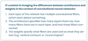
A network architecture including weights is called a model.

Sometimes, a model is pre-trained for a specific task. Other times, it is merely trained on a more general dataset, like one from ImageNet.

Such general training allows the model to learn useful features in its first layers, which can be applicable to a variety of problems and datasets. However, it can also mean that the network is not directly applicable to our problem.

Weights are usually provided as a data file specific to a given neural networks library. Multiple weights files are often provided, but they may differ in a task or in the dataset used for training.

That said, if both of these items are similar to our use case, the pre-trained network can be directly applied to the problem at hand.

Customizing architecture

If we are unable to find a suitable architecture or pre-trained network for our particular use case, then it may be a good idea to use an existing network as a starting point.

We could then apply arbitrary changes.

However, applying simple modifications to the output or input layer is the most common approach.

Output

Our simple classification example is a very good use case to illustrate why we might choose to modify the output layer.

Suppose we have a network pre-trained on an ImageNet dataset, which classifies images to one of 1,000 classes.

The images in our dataset are very similar to those on ImageNet. But the objects are different. This means the network is well trained to find features in the image, but it’s not trained in the combination of objects that characterize our classes.

If we assume we have 5 object classes, we can change the number of outputs from 1,000 to 5 — then, train the network on our dataset.

This process is called transfer learning (more about this later).

Usually, we only allow the weights in the last few layers to change and we leave the rest of them as “frozen” or fixed. The same concept can be applied to change the type of task.

We can use a neural network that’s trained to be a classifier and change the last few layers to enable it to deal with regression tasks (like predicting a value).

The key point to note is that the dataset just has to be similar.

ImageNet comprises a dataset of photographs of everyday objects. Therefore, while the convolutional filters are suitable for similar photographs, they’re unfit for application to cartoons or vector graphics, for example.

Input

Network input is another aspect we can modify, but this often requires more effort. Why?

As data flows through a network — from input to output — any upstream change may mean that the layers further down the flow become unfit for new data.

Depending on the architecture, it may be easy to change the input resolution. However, using another color model (RGB vs HSV or Lab), or changing the number of channels (like adding transparency), could also create a flood of other changes.

Some may simply mean a network has to be re-trained from scratch on the same architecture. Others may require an architectural overhaul — sometimes easy; oftentimes, very complex.

Equally, we may want to provide the network with additional features.

Each image may be accompanied by attributes that are relevant to the problem. The modern approach is to allow convolutional networks to learn the features themselves, with no help from us.

We tested this approach and, once again, the filters created by the experts outperformed the self-learned filters.

However, additional attributes may still be helpful to the main classifier (or regressor; or whatever the problem). Such assistance could come in the form of a network or algorithm, which learns some of the features that can later be processed by the classifier of the higher-order.

Such a modular construction causes the components to be networks — not a single coherent network; rather, separate networks taught via separate processes.

It’s also possible to create a classifier that captures the intermediate features, and then build the network on them. The advantage of this approach is that the classifier is easier and faster to train than a typical neural network.

Alternatively, it’s possible to go the other way.

First, we can use a ready-made network (e.g. Haystack, Betaface, Kairos) and use simple machine learning for such features. Many tools can then be used to catch features, automatically:

In Python, there’s a featuretools library, which can automatically generate features from a set of attributes;
In the scikit-learn library, there’s a SelectKBest tool, which can find a number of the best features in the classification, which we can use to reduce the space of features (if this doesn’t work, there are other methods of dimension-reduction, such as PCA).

At this point, we risk delving into the realm of custom networks, which isn’t the best bet for businesses. It’s a costly research process that requires vast knowledge and experience — not to mention a deep well of computational power.

Learning

Learning is where the magic happens. It’s just… there is no magic.

Learning is just an automated process to adjust the parameters in the network.

It’s what enables the predictions of the model to match the target labels, using the input data. Therefore, it’s what makes the network capable of solving the task.

Network Size

Neural networks can work on mobile devices, but training them is demanding: it requires a server with a powerful graphics card (or another accelerator, like a TPU or FPGA).

GPU cards are popular thanks to their computing architecture: they can be used for many simple algebraic operations at the same time, which fits into the neural network learning model.

Nvidia supplies most of the products used in computational libraries, including CUDNN for neural networks.

The length of calculations depends primarily on the number of elements in the learning set, coupled with the complexity of the problem, which translates into the rate of decrease of the learning curve.

In practice, this often means getting better prediction results from our model. However, the less clearly defined the problem, the deeper the network must be — and the more differentiating features we must find.

If we use a ready-made network for the problem (e.g. if we want to create a personalized classifier that recognizes digits, but we have a specific font), then we can take some ready-made OCR classifier (tesseract OCR, for example) and train it on a set of digits using this font.

But ready-made networks are often quite large, and their size is another variable that determines the speed of their learning: with the larger the network, the more parameters there are to learn — while the speed of learning also depends on the methodology of learning and the selected initial hyper-parameters (see section 4.6).

Large networks often come from general solutions, and their retraining is a difficult undertaking. Often, it’s a question of the level of pre-processed data that’s available.

Put another way — if we have already extracted the features from the data that differentiate the images well, then their classification isn’t so hard.

Start State

Usually, we begin under random conditions.

But if we have networks like VGG — that are very similar to our problem — and we have starting weights, then we can start with them (for example, ResNet has weights available that were learned from millions of widely available ImageNet images).

This particular dataset was supposed to be used to learn how to classify images through neural networks — it contains 1,000 classes.

Training

The actual learning process — also known as training — involves feeding the network with training data and checking the value of the loss function.

Training generates a return from the network in the form of a number — or, if an arrangement, in the form of a vector — and this number tells us how closely the result resembles a cat, a dog or a human if we’re to use our image classification example.

If the results are good, you can stop the training.

The training process consists of adjusting the weights of the network so that the network output matches its input.

The cost function is created in such a way that it checks how many training examples are classified correctly. The learning algorithm is based on backward propagation of error, using the gradient of the error function.

This loosely means it improves the weights from the output to the network input, which makes intuitive sense: if we know how much of the output is wrong, we know the extent to which we have to adjust the weights of the model.

Testing

In machine learning, the dataset is divided into several parts. Usually, the accepted method of division is k-cross-validation, which follows the below process:

We divide a dataset into ‘k’ equal parts
Then, we train and test the procedure ‘k’ times
Each time, we take a different part of the dataset as a test set
The rest, we use as a training set

K-cross-validation is a costly process.

We must train the network multiple times on different subsets of data. Therefore, in neural networks, we often prefer to use a more classical train-validate-test split.

All training is performed on a training set
Any changes to the architecture or hyper-parameters (see section 4.6) are evaluated on a validation set and the best is chosen
At the end, the final estimation of real-world performance is performed on a test set

Hyper-parameters

During the learning process, we also select some so-called hyper-parameters.

The most important hyper-parameter is the network architecture. It’s solved by taking a ready-made model from the publication to re-train on our data. Then, you just have to adjust the so-called learning rate.

We use a heuristic here; firstly, to check the fixed learning rate (e.g. between 0.001 and 0.1) to see which order of magnitude works best. Then, we adjust it precisely.

Usually, the constants are quite small.

To check the influence of the learning rate on our model, we can tweak them slightly during the learning process and plot a new learning curve as a function of error.

If the error decreases too slowly, we can reduce the learning rate during the learning process, depending on the loss function. If the inverse is true, we increase the learning rate.

Overfitting

The steps described above are used to prevent overfitting (i.e. the risk of the network learning all the training examples by heart).

Overfitting is a nightmare in machine learning.

It prevents algorithms from generalizing because they adapt too well to the training data. Generalization refers to a model’s ability to make correct predictions on new, previously unseen data (as opposed to the data used to train the model).

One of the best ways to avoid overfitting is regularization: the process of adding a term related to the inertia of weights, or a square of the magnitude of coefficients in L2, to the error function — or, by using a dropout or data augmentation technique.

Hyper-parameter Optimization

As a hyper-parameter, we can also modify the error function and its optimization (optimizing algorithms). The standard cost functions are the Euclidean norm or cross-entropy.

The latter, in particular, has an interesting property in that the cost function decreases quickly at the beginning — while the greater the initial error, the faster the network learns.

In many ways, it reflects human learning: the bigger the mistakes you make, the faster you learn.

For backward error propagation, you can choose the optimization method, with the most popular approach being AdamOptimizer, which contains the adaptive moment method.

Deploying the model to production

The ultimate goal of all our data science efforts is to create a smart model, right? Well, not exactly.

The goal is to put our model to productive use.

So, while we’ve spent the previous sections walking you through a systematic process for creating a reliable, accurate logo detection model that can theoretically solve our computer vision problem….

— Now is the time to put our model to the test.

That means putting the trained algorithm to work on an entirely new, real-world data-set, then seeing how it performs.

It is only on deployment of the machine learning model to a production environment that we find out if it really can provide accurate predictions: it is only once we expose our model to real-world data that we will know if it can add business value.

Business Requirements

When the time comes to deploy, you first need to step back and consider both your business requirements and the broader company goals; this step includes understanding existing constraints, as well as the value you’re hoping to create, and for whom.

To make this process run smoothly, consider the following questions:

Do you need to serve predictions in real-time? If yes, does real-time mean ‘within a few milliseconds’ or ‘after a second or two’?
Would predictions every 30-minutes, or just once a day after the input data is received, suffice?
How often do you expect to update your prediction models?
What will the demand be for your predictions (i.e., How much traffic do you expect)?
How much data are you dealing with?
What sort(s) of algorithms do you expect to use?
Are you in a regulated environment where the ability to audit your system is important?
How large and experienced is your team (including data scientists, engineers, and DevOps)?

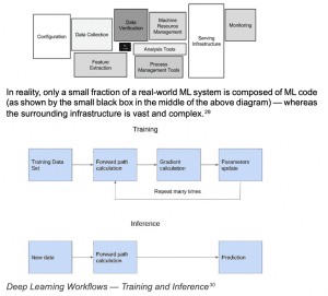
Therefore, depending on the model’s performance, size and architecture requirements, CPU, GPU, TPU accelerated, embedded or specialized hardware could be required to make adequate inferences and predictions.

Platforms

When it comes to choosing a platform, our model could be deployed on various systems, including mobile and IoT devices, embedded software, on the web, on-premises — or, in dedicated hardware.

We discuss deployment options through the remainder of this section.

Web deployments

Rest API

Serving predictions in response to canonically formatted HTTP requests
The web server runs and calls the prediction system.

Options

Deploy code to VMs, then scale by adding instances

Each instance must be provisioned with dependencies and app code
Number of instances managed manually, or via auto-scaling
Load balancer sends user traffic to the instances

Cons of VMs:

– Provisioning can be brittle

– Paying for an instance even when not in use (though auto-scaling does help)

Deploy code to containers, then scale via orchestration

App code and dependencies packaged into Docker containers
Kubernetes (or alternative — e.g., AWS Fargate) orchestrates containers (DB/workers/webservers/etc.)
Container orchestration automates the deployment, management, scaling, and networking of containers.

Cons of containers:

– Still managing your own servers and paying for uptime (not compute-time)

– However, there are fully managed inference container options in the cloud with auto-scaling so not used servers could be stopped automatically.

Deploy code as a ‘serverless function’

App code and dependencies packaged into .zip files with a single entry point function
AWS Lambda (or Google Cloud Functions/Azure Functions) manages everything else
Instant scaling up to 10,000+ requests per second, load balancing, etc.
Only pay for the compute-time.

Cons of using a ‘serverless function’:

– Entire deployment package has to fit within 500MB

– <5 min execution time

– <3GB memory (AWS Lambda)

– Only CPU execution

Model Serving

If performant inference is a requirement — be it on GPU or another supported hardware — then Model Serving becomes useful
Model servers have advantages like serving multiple models, easily loading and unloading models, and performance (because they expect models to be in optimized format after quantization, etc.)
The below are web deployment tools specialized for machine learning models:
- TensorFlow Serving, works with TensorFlow only (Google)
- Model Server for MXNet (Amazon), can also be used to serve models to the ONNX format.
- ONNX Runtime, can serve any model converted to ONNX format. There are fully managed options on Azure platform.
- Clipper (Berkley RISE Lab)
- SaaS solutions like Algorithmia

Mobile and IoT devices

Embedded and mobile devices have little memory and are slow/ expensive computers
Must reduce network size/use ‘tricks’ or quantize weights (which means reduce the number of bits that represent a number. In deep learning, this is a reduction from 32 bits: so-called full precision to 16, 8 bits or even to 4/2/1 bits is an active field of research33)

Methods for compression (discussed in 34):

Parameter pruning — can remove correlated weights and add sparsity constraints in training
Introduce structure to convolution
Knowledge distillation

If the primary use of an application is to be via mobile devices, there are several options:

TensorFlow Lite from Google (see image classification example be- low)
Core ML from Apple
PyTorch Mobile and Caffe2 from Facebook
Other options are also available

Case Study: Image Classification Using TensorFlow Lite

TensorFlow Lite is an open source, deep learning framework for on-device inference. The framework can access optimized models that support both common mobile use cases as well as less typical edge-cases — such as image classification or object detection.

With Tensorflow Lite, we use and optimize pre-trained models to identify hundreds of classes of objects: including people, activities, animals, plants, and places.

Google provides starter image classification models with accompanied labels capable of learning how to use image classification models within a mobile app. Once we have the starter model up-and-running on our target device, we can experiment with different models to find the optimal balance between performance, accuracy, and model size.

To perform an inference — the process of predicting the class — we pass an image as an input into the model, which then produces, as its output, an array of probabilities between 0 and 1 (each numerical output corresponds to a label in our training data).

TensorFlow offers a large number of image classification models, so you should aim to find the model that best suits your application based on performance, accuracy, and model size (note: there are trade offs in choosing one over another).

Performance

Performance refers to the amount of time it takes for a model to run an inference on a given piece of hardware: less time = better performance.

The performance you require depends on your application.

Performance can be important for applications like real-time video where it may be necessary to analyze each frame in the time before the next frame is drawn (e.g. inference must be faster than 33ms to perform real-time inference on a 30fps video stream)
TensorFlow Lite quantized MobileNet models’ Top-5 accuracy ranges from 64.4 to 89.9%

Size

The size of a model when on-disk varies with its performance and accuracy.

Size may be important for mobile development where it can impact app download sizes; or when working with hardware where available storage can be limited
Tensorflow Lite quantized MobileNet models’ size ranges from 0.5 to 3.4 Mb

Architecture

TensorFlow Lite provides several different models of architectures: for example, you can choose between MobileNet or Inception — among others.

The architecture of a model impacts it’s performance, accuracy, and size
All TensorFlow-hosted models are trained on the same data, meaning you can use the available statistics as a fair comparison when choosing which model is optimal for your application

Customized model

We can also use a technique known as transfer learning to re-train a model to recognize classes specific to our data.

Cloud

There are a host of cloud computing providers available, including Google Cloud Platform, Microsoft Azure, and Amazon AWS, among others.

Cloud computing providers can host your models so that you can draw predictions straight from the cloud. The process of hosting a saved model is called deployment and an example of using a Google service (Google AI Platform) is presented below.

Google AI Platform

Google AI Platform provides the tools to take a trained model to production and deployment; while its integrated tool chain helps you build and run your own machine learning applications.

Google AI Platform also supports Kuberflow — Google’s very own open source platform — which means you can build portable ML pipelines to run on-premises, or on Google Cloud, without significant code changes.

The platform also provides access to other Google AI technology like TensorFlow, TPUs and TFX tools as you deploy your AI application to production.

Plus, you can use the platform prediction services to deploy your models to production on GCPs in a serverless environment; or, you can do so on-premises using the training and prediction microservices provided by Kubeflow.

Amazon SageMaker

Amazon SageMaker is a fully-managed service that provides developers and data scientists with the ability to build, train and deploy machine learning models (ML) more easily than in traditional ML development.

SageMaker provides all of the components used for machine learning in a single toolset: labelling, building, training & tuning and deployment & management.

Amazon Elastic Inference

Amazon Elastic Inference allows developers to attach low-cost GPU-powered acceleration to Amazon EC2 and Sagemaker instances or Amazon ECS tasks, to reduce the cost of running a deep learning inference.

Amazon Elastic Inference supports TensorFlow, Apache MXNet, PyTorch and ONNX models.

Amazon Elastic Inference also allows developers to attach just the right amount of GPU-powered inference acceleration with no code changes, so you can choose the CPU instance in AWS that’s best-suited to the overall computing and memory needs of your application, and then separately configure the right amount of GPU-powered inference acceleration, allowing you to leverage resources efficiently and reduce costs.

The amount of inference acceleration can be scaled up and down using Amazon EC2 Auto Scaling groups to meet the demands of an application without over-provisioning capacity.

EC2 Auto Scaling increases your EC2 instances to meet increasing demand, while it also automatically scales up the attached accelerator for each instance. Similarly, when it reduces your EC2 instances as demand goes down, it automatically scales down the attached accelerator for each instance.

This helps to pay only for what is needed and when it’s needed.

Embedded

For embedded devices, Nvidia Jetson is a specific low-power GPU. At just 70 x 45 mm, it is a production-ready System on Module (SOM) that can deploy AI directly to devices.

The Jetson Nano delivers 472 GFLOPs to run AI algorithms: it can run multiple neural networks in parallel. Plus, it can process high-resolution sensors simultaneously.

For detailed specifications, see the Nvidia website.

On-premises

If data privacy requirements (or another consideration, e.g., cost) force you not to use cloud-based infrastructure, you can deploy our model using on-premises infrastructure.

Dedicated hardware

If speed or size are the most important characteristics; then specialized, dedicated hardware solutions will be helpful.

Habana supplies purpose-built devices that make AI Training and AI Inference fast: the Habana Goya Inference Processor runs inference on ResNet-50 with a speed of 15,000 images per second on image classification tasks. Habana’s Goya is a class of programmable AI processors, designed from the bottom-up for deep neural network workloads: particularly those dedicated to inference workloads.

As per Habana, the HL-1000 processor is the first commercially available, deep learning inference processor designed specifically for delivering high performance and power efficiency.

It supports most leading deep learning frameworks — including TensorFlow, MXNet, Caffe2, Microsoft Cognitive Toolkit, PyTorch and ONNX45 model format (deep learning frameworks can be exported to ONNX for- mat and then served using some ONNX runtime).

Continuous Deployment

Continuous Integration (CI) and Continuous Deployment (CD) tools are a critical aspect in mitigating the risks of ML systems.

Sometimes, the application of DevOps principles to ML systems is called MLOps. MLOps aims to unify ML systems development (Dev) and ML system operation (Ops) and includes the automation and monitoring of all steps of ML system construction — including integration, testing, deployment and infrastructure management.

Some challenges of setting up proper CI and CD include:

Team skills — ML researchers may not be experienced software engineers capable of building production-class services.
Development — Tracking different features, algorithms, architectures, and hyperparameters to find what worked and what didn’t.
Testing — In addition to typical unit and integration tests, data validation, trained model quality evaluation and model validation are needed.
Deployment — ML systems may require deployment of a multi-step pipeline to retrain and deploy models automatically.
Production — Due to constantly evolving data profiles, ML models can have reduced performance. Therefore you need to track summary statistics of your data and continuously monitor the online performance of your model.

The most common level of MLOps maturity involves manual process; the highest level involves automating both ML and CI/CD pipelines.

Automation is essential for the rapid and reliable update of the pipelines in production. An automated CI/CD system also lets data scientists rapidly explore new ideas around feature engineering, model architecture, and hyper-parameters.

They can then implement these ideas and automatically build, test, and deploy the new pipeline components to the target environment — if you’re interested in MLOps, the setup requires these components:

Source control
Test and build services
Deployment services
Model registry
Feature store
ML metadata store
ML pipeline orchestrator

To summarize, implementing ML in a production environment doesn’t only mean deploying your model as an API for prediction. Rather, it means deploying an ML pipeline that can automate the retraining and deployment of new models.

Setting up a CI/CD system enables you to automatically test and deploy new pipeline implementations. While the system also lets you cope with rapid changes in your data and business environment.

But worry not.

You don’t have to move all of your processes from one level to another immediately. You can gradually implement these practices to help im- prove the automation of your ML system in both development and production.

Unit/Integration Tests

These are tests both for individual module functionality and for the entire system.

Continuous Integration

These are tests that run every time new code is pushed to the repository — and before deployment of the updated model.

SaaS For Continuous Integration

CircleCI/Travis
- Integrate with your repository: every push kicks off a cloud job
- Job can be defined as commands in a Docker container, and can store results for later review
- No GPUs
- CircleCI has a free plan
Jenkins/Buildkite
- Nice options for running CI on your own hardware, in the cloud, or mixed
- Good options for the nightly training test (can use your GPUs)
- Ultra-flexible

Containerization (via Docker)

A self-enclosed environment for running the tests.

No OS = lightweight
Lightweight = heavy use
Container orchestration: Kubernetes is the open source winner, but cloud providers have good offerings, too.

ONNX

Open Neural Network Exchange (ONNX) is an open source format for deep learning models. It supports different frameworks, including frameworks that are suited to development — PyTorch being one example — but that don’t necessarily have to be good at inference (Caffe2 for example).

Models in ONNX can be deployed on Android and iOS. A custom serving of ONNX models is found here.

ONNX is a counterpart to TensorFlow and can run on any Linux server. It is also a subcomponent of Windows 10. Azure and Amazon (AWS Sage- Maker) have the capability to deploy managed ONNX models.

Monitoring and optimizing performance

Once the model is deployed, it’s critical to monitor its performance over time. This is a crucial phase of the machine learning life-cycle. There are two goals of monitoring:

To check the model is served correctly
To check the performance stays within limits over time

How and what to monitor

It’s good practice to automate the monitoring process. And to provide visualisations performance over time. Monitoring should calculate performance and send alerts when metrics slip beyond pre-defined limits.

Metrics to monitor may include:

Model predictions on the test set, with known ground truth values
The number of model servings per time period

Setting the necessary alerts requires fine-tuning the monitoring service to avoid overwhelming users with a flux of unnecessary performance warnings.

At the same time, it’s important to ensure all critical alerts arrive as needed. Another important factor to take into account is the model performance degradation owing to concept drift.

To account for this, monitoring could include:

Randomly collecting inputs
Analyzing the inputs and assigning the labels
Comparing the ground truth labels with the model predictions
Generating alerts where there is a significant difference

As a rule of thumb: a dozen examples per class is the recommended number for model performance checks. As for the frequency, we suggest analyzing the past model performance for issues, tracing the speed at which new data arrives.

To allow for the entire model monitoring process to be traceable, the events of monitoring tasks must be logged.

Besides tracking obvious metrics like accuracy, precision or recall, it’s also worth monitoring change over time — also known as ‘prediction bias.’

Prediction bias is when the distribution of predicted classes does not closely match the distribution of observed classes. It can mean that the distribution of the labels in the training data and the current distribution of classes in production are different, which indicates a possible change that needs investigation.

If low performance is detected, it may mean retraining the model with new images.

How to optimize performance

To maintain and optimize a model’s accuracy in production, there are several key steps to follow:

1. Retrain production models Frequently: To capture evolving and emerging patterns, you need to retrain your model with the most re- cent data

• For example, if your app recommends fashion products using ML, its recommendations should adapt to the latest trends and products.

2. Continuously experiment with new implementations to produce the model: To harness the latest ideas and advances in technology, you need to try out new implementations, such as feature engineering, model architecture, and hyperparameters.

• For example, if you use computer vision in face detection, face patterns are fixed, but emerging techniques can improve the detection accuracy.

A selection of available solutions

Amazon SageMaker

Amazon SageMaker continuously monitors the quality of Amazon SageMaker machine learning models in production. It enables developers to set alerts for when there are deviations in the model quality, such as data drift.

Early and proactive detection of these deviations enables you to take corrective actions, such as retraining models, auditing upstream systems, or fixing data quality issues without having to monitor models manually or build additional tooling.

You can use Model Monitor pre-built monitoring capabilities that do not require coding. While you also have the flexibility to monitor models by coding custom analysis.

Amazon Augmented AI

Amazon Augmented AI (Amazon A2I) provides tools to build the workflows required for human review of ML predictions.

Google Continuous evaluation

Google Continuous evaluation regularly samples prediction input and output from trained and deployed machine learning models. An AI Platform Data Labeling Service then assigns human reviewers to provide ground truth labels for your prediction input; alternatively, you can pro-vide your own ground truth labels.

The Data Labeling Service compares your models’ predictions with the ground truth labels to provide continual feedback on how your model is performing over time.

Microsoft Azure Machine Learning

Microsoft Azure Machine Learning allows you to collect input model data. Once collection is enabled, the data you collect can help you to:

Monitor data drift
Make decisions if and when to retrain your model
Retrain models with newly collected data

With Azure Machine Learning, you can monitor data drift as the service sends email alerts whenever it detects a drift.