Big Medical Image Preprocessing With Apache Beam | A Step-by-Step Guide

Using artificial intelligence in healthcare is fraught with challenges. 

A unique problem in the field is heavy input formats. Tissue samples are often digitalized in ultra-high resolution. And the file size of these images can be several gigabytes, making them impossible to load in a generic image viewer (due to a lack of memory to accommodate a deserialized image). 

That’s why we must pay particular attention to preprocessing when using particularly large images with any artificial intelligence model. This article will walk you through how to process large medical images efficiently using Apache Beam — and we’ll use a specific example to explore the following:

• How to approach using huge images in ML/AI
• Different libraries for dealing with said images
• How to create efficient parallel processing pipelines

Ready for some serious knowledge-sharing? 

Let’s get started!

Background: Mayo Clinic STRIP AI competition

This article is based on our recent experience at the Mayo Clinic STRIP AI competition organized by Kaggle.

Kaggle is an online community for data scientists that regularly organizes data science contests. In each contest, participants get a problem and an associated dataset before being tasked with creating a model that best solves the issue at hand. 

The solutions are then ranked, and the top competitors receive a prize. Often, the problems come from external entities trying to use the community to find proof of concept AI solutions to problems in their domain. One such entity is The Mayo Clinic: a non-profit American academic medical center focused on integrated healthcare, education, and research.

The Mayo Clinic sponsored the Mayo Clinic – STRIP AI competition focused on image classification of stroke blood clot origin. The goal was to classify the blood clot origins in an ischemic stroke. Using whole-slide digital pathology images, participants had to build a model that differentiates between the two major acute ischemic stroke etiology subtypes: cardiac and large artery atherosclerosis.

The standard treatment for an acute ischemic stroke is mechanical thrombectomy (clot removal). After the occlusion is extracted from the patient’s blood vessel, it is possible to analyze the tissue sample. The tissue is scanned in high resolution and digitalized. A healthcare professional (using dedicated viewer software) can then use the scans to determine the stroke etiology and clot origin, which helps treat the patient and prevent future strokes.

But it’s not easy to spot the tell-tale signs in scans. That’s why the clinic wants to harness the power of deep learning in a bid to help healthcare professionals in an automated way. Unfortunately, the competition rules prevent us from publishing competition data publicly. 

So while you won’t see exact samples, you can find a blood clot scan sample below (taken from Orbit image analysis machine learning software, used for the histological quantification of acute ischemic stroke blood clots).

A, C: Histopathological staining of an AIS clot with H&E stain, 1X & 10X respectively

Preprocessing challenges

Before data scientists can apply deep learning to the tissue samples, the data needs to be preprocessed. Typical Neural Network architectures take relatively small images (for example, EfficientNetB0 224x224 pixels) as input. This is not compatible with the image sizes of the images in the original dataset, which can reach tens of thousands by tens of thousands of pixels.

The preprocessing had to extract meaningful data from the source images while still being lightweight enough to run on Kaggle infrastructure within a limited time. We decided to implement the same preprocessing pipeline for training and inference to ensure we didn’t introduce any skew.

The challenges that we faced with preprocessing included the following:

• 395.36 GB of TIFF files as input
• TIFF files that were several GB in size
• Inference had to run on limited Kaggle instances (16GB RAM, 4 CPU, 20 GB persistent disk space)
• Inference had to run within a limited submission time (9 hours for about 280 images)
• Preprocessing should be shared for training and inference (the training set had 754 images)

Due to the above factors, we were forced to use the machine’s CPU to the maximum while limiting memory usage. Apache Beam helped us parallelize our computations. libvips and openslide helped us deal with the huge image files.

The pipeline

Dataset structure

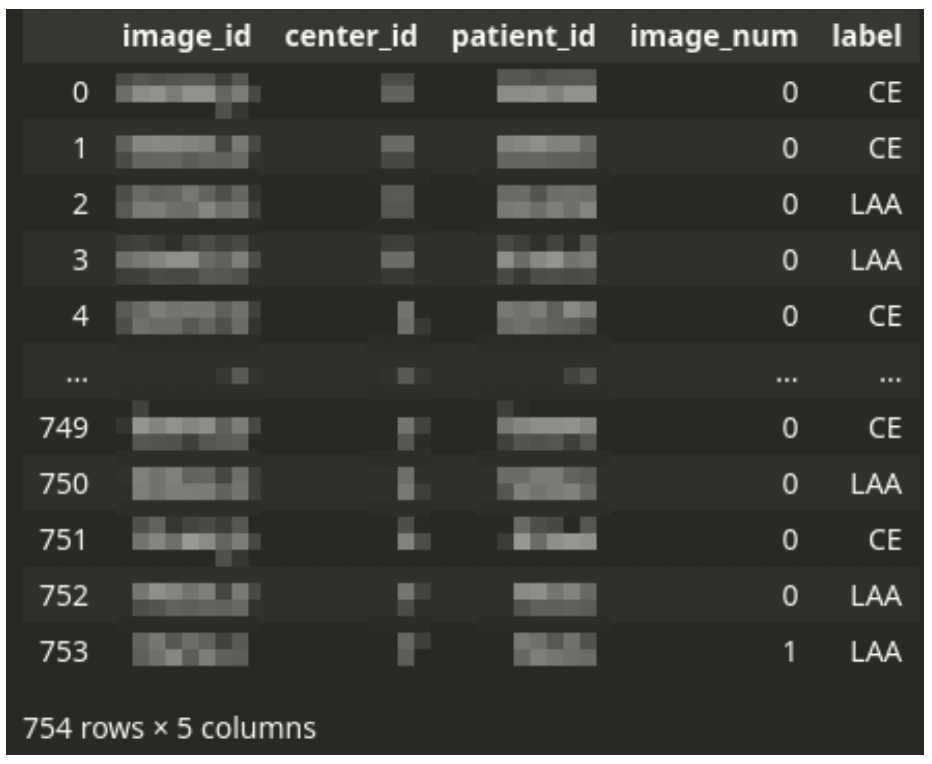
Censored training CSV file structure

The main CSV file drives the dataset. The CSV file contains one row for each tissue image scan. Each patient can have one or a few images.

There is always a single diagnosis, even from multiple images – the stroke subtype is assigned to a patient, not an image. Thus the dataset needs to be logically grouped by patient ID.

The CSV file is accompanied by a set of large TIFF images. Each image corresponds to a single row in the CSV file. The TIFF files contain digital scans of tissue slices. A single image can have multiple fragments of tissue. There is usually a large area of the background. The background is not always a solid color – sometimes, there might be a pattern of a different color.

The images contain large useless background areas that are a prime target for dimensionality reduction – we will want to discard the background areas from further processing as they carry no helpful information.

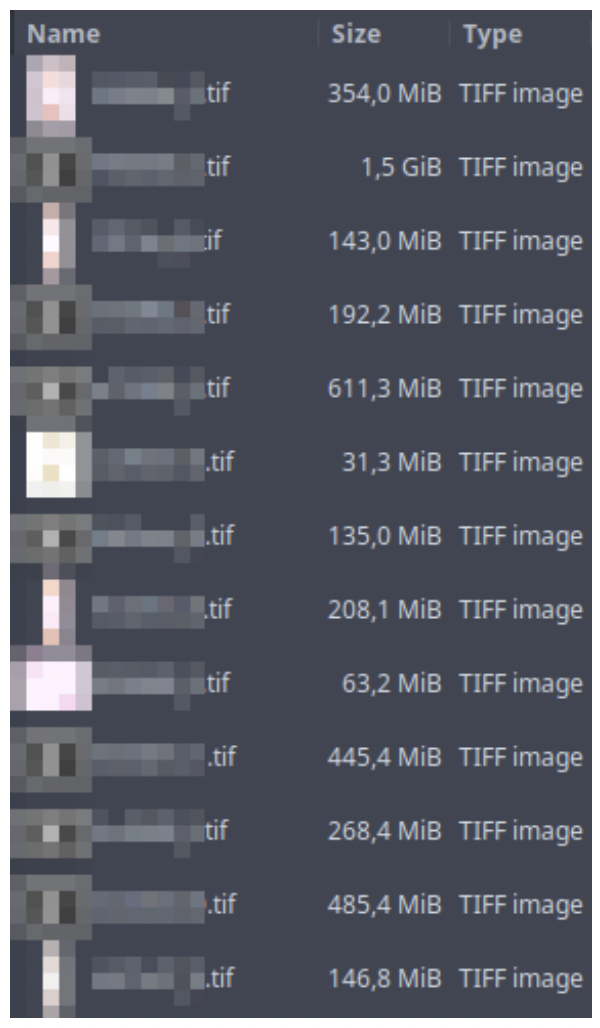
Censored fragment of images directory listing

Multiple Instance Learning

One patient can have multiple images but a single diagnosis in the dataset. The patient’s data (patient ID, ID of medical center, and the diagnosis label) are duplicated across multiple image rows if the patient has more than one image.

This problem can be tackled by an approach called Multiple Instance Learning. In classical supervised learning, each observation gets a label, and an ML model is trained on observations. In Multiple Instance Learning, that label is not assigned to an observation but to a bag of observations. If any of the observations in a bag has a positive label, the whole bag is considered positive. Otherwise, the entire bag is considered negative. The model is trained on bags of observations.

We can well explain this in a cancer detection example. Imagine that there is a patient that we suspect of having cancer. We take a few tissue samples from the patient from different places. We want to determine whether the patient has cancer or not. We analyze all the samples. If any of the samples we check show signs of cancer, we diagnose the patient as having cancer. On the other hand, to diagnose the patient as cancer-free, we need to determine that none of the samples show signs of cancer.

In the case of our competition problem, a single diagnosis for the patient is provided for a bag of the patient’s images. The dataset structure does not allow us to determine diagnostically relevant images. We want to take the Multiple Instance Learning idea even further in our approach. The raw input images are too big to use for processing directly. The diagnosis is performed by a medical professional by looking at the image while zoomed-in rather than by having an overlook of the whole sample. 

The diagnosis can be made by looking at microscopic structures inside the tissue. Our modeling solution would be to present an ML model with a bag of zoomed-in tiles generated from multiple images of a single patient and a common diagnostic label. The model would be able to learn not only to find the tell-tale signs on a given tile but also to choose which of the tiles are diagnostically relevant.

Train-test split

We split the training dataset into the following groups:

• Training split ( ~80% patients)
• Validation split (~10% patients)
• Evaluation split (~10% patients)

We ensure that multiple images of a single patient’s tissues are always together in the same split. While splitting, we use stratification by medical center ID, trying to have an equal representation of images from a given location in each split.

The splitting process outputs a few CSV files with the same structure as the original input CSV file.

Inference target

During inference (when making predictions), we had to predict the probabilities of the stroke having each of the two subtypes (CE – Cardioembolic and LAA – Large Artery Atherosclerosis) per patient.

Concept

The diagram illustrates the conceptual flow of data through our preprocessing pipeline:

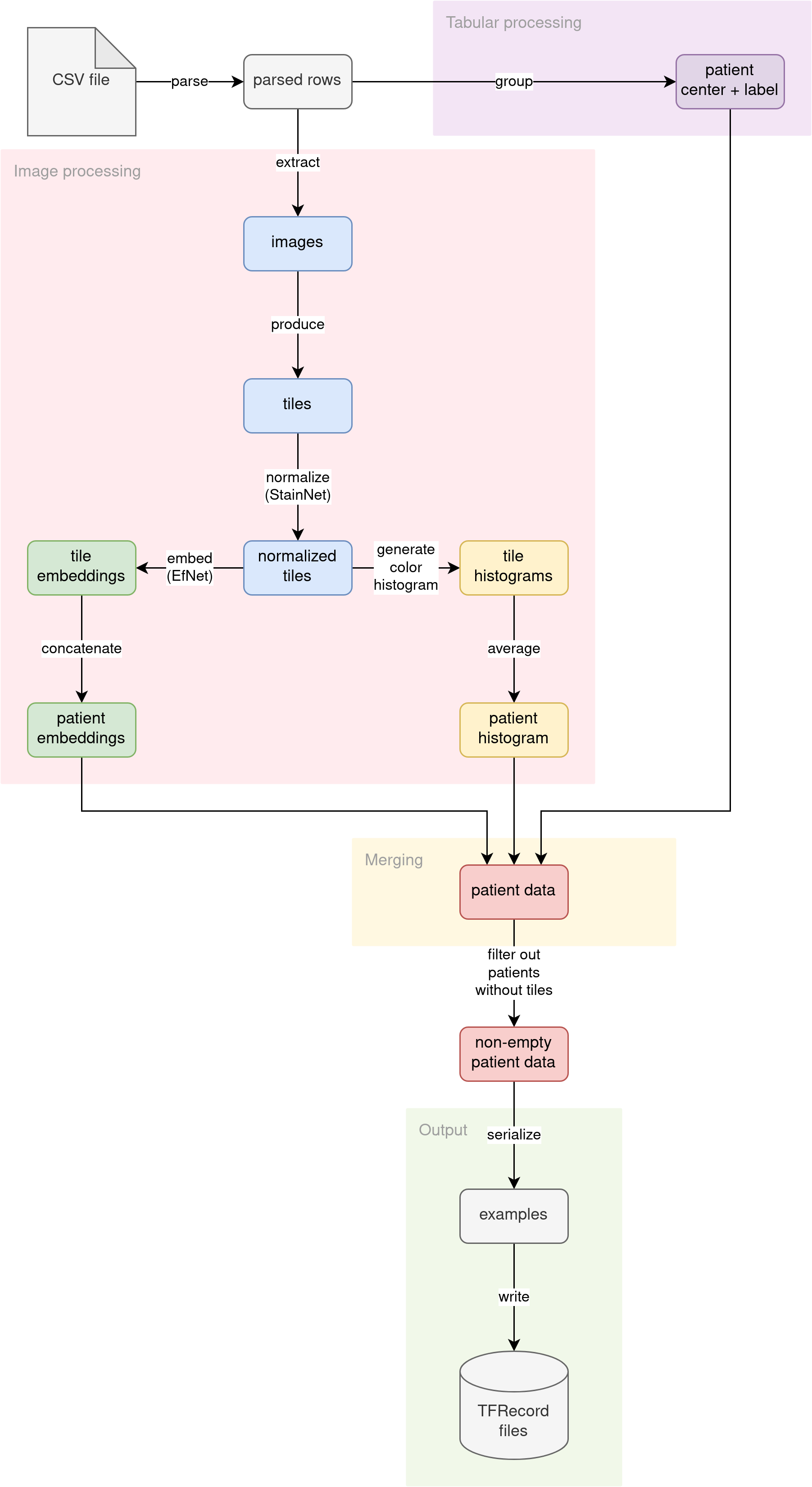
Pre-processing pipeline concept

Parse CSV

The source CSV file (no matter if the training file with labels or the inference file without labels) is read into lines. The lines are then parsed into pythonic dictionaries. Patient ID is used as the key. Multiple images per patient are not grouped yet. This step prepares the fundamental building block for the rest of the pipeline.

Further down the pipeline, processing diverges into two streams:

• Tabular data processing
• Image data processing

Tabular data processing

The patient tabular attributes (ID of the medical center where the patient was admitted and optional diagnosis label) are grouped. Since the diagnosis is determined per patient, we are grouping the data by patient ID. The attributes (medical center ID and diagnosis label) should match across multiple patient images.

Image data processing

The primary source of information for this problem is the images themselves. We decided to analyze the images in the following ways:

• Split the image into tiles and use tiles as input to a computer vision model
• Extract histograms of colors in images

Tile generation

The raw TIFF input images are too big to use for processing directly. We decided to go with the Multiple Instance Learning approach, where we feed a model with a bag of zoomed-in image tiles so that the diagnosis can be made by looking at microscopic structures inside the tissue.

The tiles are going to be generated from all patient’s images. There will be a single label for the whole bag. We decided to split each raw input image into smaller tiles (448x448 pixels) and feed the subsequent ML models with a set of small tiles downsized only to half of the original tile size (224x224 pixels – that means a 50% zoom level as compared to the raw image).

The raw input images are large, but they contain extensive sections of the background. In most images, there is much more background than the actual tissue. We wanted to limit further processing to only parts of the image that contained solid tissue. To that end, we filter out tiles containing too much background.

We downscale the original raw image to make it suitable for analysis. Then, we divide it into tiles. For each tile, we analyze the scaled-down version and check the percentage of the tile’s pixels detected as background. Different images from the dataset have different background colors (not always pure white). 

We assumed that very bright pixels (over 190 on all 3 RGB channels) contain a background. If the tile had more than 10% pixels marked as background, we would discard it from further processing, leaving only tiles that contain >90% tissue.

This approach enabled us to generate a subset of tissue-only tiles from each image with 50% zoom.

Tile normalization

We noticed that the raw images had different color schemes. Some were pinkish, some yellowish, and others greenish. We decided to use StainNet to normalize all images before further processing. Since StainNet produces coloring consistent across multiple tiles of the same image, we could apply the pre-trained StainNet Neural Network on batches of random tiles.

Tile embedding

Computer vision is a complex problem. Training Convolutional Neural Networks for image classification is time and resource-intensive. 

Instead of starting from scratch, we applied a technique called transfer learning by using a pre-trained EfficientNet neural network to generate tile embeddings. We ran each normalized tile through the pre-trained EfficientNet B0 model without top layers. The neural network generated a [7, 7, 1280]-shape embedding for each tile. 

Thinking that the position of tissue structure in the tile is not relevant to solving the problem, we decided to aggregate the embeddings across the [7, 7]-shape image to produce a single 1280-dimensional embedding vector. We generated both max and mean aggregations and left it up to the subsequent model to pick which of those it wanted to use as input.

Finally, for each patient, we generate two vectors:

• • avg – mean-aggregated embeddings of shape [<number of tiles per patient>, 1280]*

• • max – max-aggregated embeddings of shape [<number of tiles per patient>, 1280]*

*where <number of tiles per patient> is a ragged dimension whose size depends on the number of tiles generated per patient.

The generated embedding vectors are much smaller in size than the original images. They take up less disk space and enable us to cache the whole dataset for more efficient training.

Color histograms

Thinking that different colors of pixels in the tissue sample correspond to different microscopic structures, we figured out that the proportion of given structures per tile might be an indicative diagnostic feature. We decided that we could express the proportions by calculating color histograms for all pixels in the image. We generate a [16, 16, 16]-shape histogram for each normalized tile.

Since there are multiple tiles per patient and we wanted to analyze the overall distribution of microscopic structures, we are averaging the histograms along all tiles generated from all user’s images. The aggregation produces a single vector of shape [16, 16, 16] for a patient. This histogram vector becomes another input available to subsequent models.

Merging

We have three independent streams of features per patient, calculated by different parts of the pipeline:

• A single color histogram (shape [16, 16, 16])
• Multiple tile embeddings per patient (two aggregations, each shape [<number of tiles per patient>, 1280])
• 2 tabular features (medical center ID and optional diagnosis label) per patient (each a scalar value)

In the merging phase of preprocessing, we connect all of these features into a single entity, using patient ID as the join key.

Output

The pipeline converts the joined features into Tensorflow’s tf.train.Examples. Then, the serialized Examples are written to a set of TFRecord files. Those TFRecord files can later be loaded by the model training code or inference code as datasets. The generated datasets are much smaller in disk size than the original raw images (from ~400 GB, we distill ~2.2 GB datasets).

Apache Beam: the tool used for medical image processing

To tackle the implementation of the complex preprocessing pipeline, we used Apache Beam. Apache Beam is an open-source framework that provides a unified programming model for batch and streaming data processing pipelines. 

The framework simplifies the implementation of large-scale data processing. Beam supports a large set of input and output formats. The processing pipeline written using Apache Beam can be executed both locally as well as scaled up on the cloud (for example, using Dataflow on the Google Cloud Platform).

We used Apache Beam for the following reasons:

• We have a complex pipeline with three parallel streams of work and a merging phase that can be nicely expressed using Beam SDK
• Beam supports text inputs (CSV file)
• Beam supports TFRecord sinks
• Beam transparently supports Google Cloud Storage (where we kept our data)
• Beam can run locally, taking full advantage of multiprocessing, efficiently using all locally available processing power (useful for Kaggle submissions with limited allowed run time)

Apache Beam is a building block of other production-ready tools. For example, many Tensorflow Extended components use Beam under the hood.

Processing large medical images

Handling large TIFF input images cannot be implemented using standard Python tools for image loading (PIL) simply because of memory constraints.

An example RGB input image of size 46177 by 77440 pixels would take  46177 * 77440 * 3 = 10 727 840 640 bytes – almost 11 GB! There are even bigger images in the training set. When paired with Kaggle instances having 16 GB of RAM, one can easily see that loading the whole image into memory is a no-go.

Instead, we need to use other third-party libraries that would be able to operate on the huge TIFF images without loading them whole into memory. 

We used two such libraries:

• libvips – to efficiently load down-scaled versions of input images to perform background analysis
• openslide – to efficiently extract only the interesting tiles (filled chiefly with tissue) of the original image in original resolution

Using libvips to load down-scaled versions of large images

We decided to down-scale the input images by a factor of 16. For the previous sample image, the memory needed to store the smaller version of the image is only (46177/16) * (77440/16) * 3 = 41 940 720  bytes (less than 42 MB, compared to ~11 GB for the full version).

import numpy as np
from numpy import typing as npt
import pyvips


def load_downscaled_image(
    local_file_path: str,
    downsample_ratio: int = 16,
) -> npt.NDArray[np.uint8]:
    full_img = pyvips.Image.new_from_file(local_file_path)
    scaled_down_image: npt.NDArray[np.uint8] = full_img.resize(
        1 / downsample_ratio
    ).numpy()
    return scaled_down_image
    

Using the code above,  libvips will load and downscale the image on the fly without loading the full version. The return value will contain a NumPy array of unsigned 8-bit integers with scaled image contents.

Please note that the  libvips API creates an image processing pipeline. Using new_from_file only loads image metadata. Same thing with resize: no actual resizing is performed. The constructed pipeline is executed only at the moment of explicit materialization – upon calling numpy().

Using openslide to extract certain tiles from large images

In the previous section, we described how we could load a scaled-down version of a large image for analysis. Upon determining which square tiles of the image contain mostly tissue, we wanted to extract the contents of those tiles in the original resolution.

Since we wanted to use EfficientNet B0 in later steps, we needed the input images to have 224 by 224 resolution (required input shape for EfNet). We decided to load tiles twice as big (224 * 2 = 448 pixels in size) for preprocessing and scale them down by a factor of 2 just before embedding them using EfNet.

Each RGB tile extracted would take up (224 * 2) * (224 * 2) * 3 = 602 112  bytes of memory (~600 KB).

The code below shows how one can use openslide to load only specific tiles from a large image:

from typing import Tuple, Sequence, Iterable

import openslide
from PIL import Image


def extract_tiles(
    input_image_path: str,
    non_empty_tile_indices: Sequence[Tuple[int, int]],
    tile_size: int = 224 * 2
) -> Iterable[Image]:
    size = (tile_size, tile_size)
    with openslide.open_slide(input_image_path) as slide:
        for row, column in non_empty_tile_indices:
            left = column * tile_size
            top = row * tile_size
            position = (left, top)
            # Extract the tile from the original image
            # in original resolution.
            tile_img = slide.read_region(
                position, 0, size
            ).convert("RGB")  # convert from RGBA to RGB
            yield tile_img

A tile loaded in this fashion is a PIL image. We can convert it into a NumPy array of unsigned 8-bit integers using the following:

import numpy as np
from numpy import typing as npt


img_array: npt.NDArray[np.uint8] = np.array(tile_img)

Please note that the tile extraction snippet does not materialize all the extracted tiles. Instead, the function is a generator that materializes one tile at a time. This approach enables us to keep memory usage low (even though, from some images, we are extracting thousands of tiles) and integrates well with Apache Beam.

Applying model predictions

In our preprocessing pipeline, we have two places where we are executing inference using pre-trained models:

• In raw tile normalization (StainNet)
• In normalized tile embedding (EfficientNet)

It’s straightforward to implement ML inference in Apache Beam. A ModelHandler class is provided in the apache_beam.ml.inference.base package that can wrap an ML model for inference. It is framework-agnostic and can be applied to any ML model. 

The class is defined as a generic:

class ModelHandler(Generic[ExampleT, PredictionT, ModelT]):
    ...

Where the type variables have the following meaning:

• ExampleT – the type of incoming examples
• PredictionT – the type of outgoing predictions
• ModelT – the type of ML model loaded and used for generating predictions.

To use the ModelHandler, one needs to create a class that inherits from it with concrete types and implement two methods:

• load and initialize a model for processing:

  def load_model(self) -> ModelT:
      ...

• run inference on a batch of examples:

  def run_inference(
      self,
      batch: Sequence[ExampleT],
      model: ModelT,
      inference_args: Optional[Dict[str, Any]] = None
  ) -> Iterable[PredictionT]:
      ...

An inference wrapper defined in the following way can be easily integrated into an Apache Beam pipeline (see pipeline implementation snippet in the following section). Beam will automatically take care of batching incoming examples (it will determine the optimal batch size) and loading a single model instance per node.

Below you can find a snippet that shows how to apply ModelHandler to execute tile embedding using EfficientNet in TensorFlow:

from typing import (
    Iterable
    NamedTuple,
    NewType,
    Sequence,
)

from apache_beam.ml.inference.base import ModelHandler
import numpy as np
from numpy import typing as npt
import tensorflow as tf


# alias type for string patient ID
PatientId = NewType("PatientId", str)
# alias for NumPy tile as an array
#  of 8-bit unsigned integers
Image = npt.NDArray[np.uint8]


class TileEntry(NamedTuple):
    """Schema for a tile entry."""

    patient_id: PatientId
    image: Image


class Embedding(NamedTuple):
    """Schema for aggregated embeddings."""

    max_embedding: tf.Tensor
    avg_embedding: tf.Tensor


class EmbeddingEntry(NamedTuple):
    """Schema for prediction entry."""

    patient_id: PatientId
    embedding: Embedding


def embed_tiles(
    model: tf.keras.Model,
    tiles_batch: Sequence[Image],
) -> Iterable[Embedding]:
    """
    Run a batch of input images through EfNet
    to generate aggregated embeddings.
    """
    # convert from NumPy to TensorFlow
    input_tensor = tf.ensure_shape(
        tf.convert_to_tensor(tiles_batch),
        [None, 224 * 2, 224 * 2, 3],
    )
    # The input tile is twice as big as needed
    # for EfNet - we scaled it down 2x here.
    resized_input_tensor = tf.image.resize(input_tensor, [224, 224])
    # generate embeddings using EfNet
    results = model(resized_input_tensor, training=False)
    avg_embeddings = tf.ensure_shape(results["avg"], [None, 1280])
    max_embeddings = tf.ensure_shape(results["max"], [None, 1280])
    # wrap the results
    for avg_embedding, max_embedding in zip(avg_embeddings, max_embeddings):
        yield Embedding(avg_embedding=avg_embedding, max_embedding=max_embedding)


class TileEmbeddingModelHandler(
    ModelHandler[TileEntry, EmbeddingEntry, tf.keras.Model]
):
    """Wrapper around EfficientNet embedding."""

    def load_model(self) -> tf.keras.Model:
        """Prepare an EfNet aggregation model for tile images."""
        # The model will consume 224x224 RGB images
        image = tf.keras.layers.Input(
            shape=(224, 224, 3), name="image", dtype=tf.float32
        )
        # We use EfNet B0 without top layers for embedding
        backbone = tf.keras.applications.EfficientNetB0(
            include_top=False, weights="imagenet", input_tensor=image
        )
        # To save on compute resources, we won't fine-tune the EfNet backbone
        backbone.trainable = False
        # The backbone output has shape [<batch size>, 7, 7, 1280]
        # We generate two aggregations over the backbone output
        # to obtain a [<batch size>, 1280] shape
        avg_pool = tf.keras.layers.GlobalAveragePooling2D()(backbone.output)
        max_pool = tf.keras.layers.GlobalMaxPooling2D()(backbone.output)
        model = tf.keras.Model(
            image, {"avg": avg_pool, "max": max_pool}, name="EfficientNet"
        )
        model.compile()
        return model

    def run_inference(
        self,
        batch: Sequence[TileEntry],
        model: tf.keras.Model,
        inference_args: Optional[Dict[str, Any]] = None,
    ) -> Iterable[EmbeddingEntry]:
        """Run inference using the loaded model."""
        # Extract just the tile images from the input batch
        input_images = [tile.image for tile in batch]
        # Embed tile images using EfNet
        embeddings = embed_tiles(model, input_images)
        # Wrap the resulting embeddings together with the patient identifier
        for tile, embedding in zip(batch, embeddings):
            yield EmbeddingEntry(patient_id=tile.patient_id, embedding=embedding)

Pipeline implementation

Our preprocessing pipeline is rather complex, with multiple parallel streams of processing. If we wanted to express that in pure Python, we would end up with a very complex code. Luckily, we can use Apache Beam to define and run the complex pipeline relatively easily.

Beam pipeline syntax

To create a pipeline, one needs to use Pipeline from apache_beam (the module is customarily aliased as just beam), preferably as a context manager:

with beam.Pipeline(options=beam_options) as pipeline:
    ...

To connect operations, one uses the pipe operator (|):

filenames = pipeline | beam.Create([input_csv_path])
csv_dicts = filenames | beam.FlatMap(read_csv_lines)
parsed_rows = csv_dicts | beam.Map(parse_row)

Each operation can optionally get a descriptive name (this is required if types of operations in the pipeline are not unique) using the right bit shift operator (>>):

filenames = pipeline | "Create" >> beam.Create([input_csv_path])
csv_dicts = filenames | "ParseCSV" >> beam.FlatMap(read_csv_lines)
parsed_rows = csv_dicts | "ParseRows" >> beam.Map(parse_row)

The pipeline must be comprised of Beam transforms customized with custom callbacks (see Beam Programming Guide).

Beam can read data from different sources. In our pipeline, we use the Create operation to import a data seed into our Beam pipeline. The op creates a collection that can be further processed.

Elements processed with a Beam pipeline can be of any serializable type. Beam can use tuples as keyed elements, where the first element of the tuple is considered to be the key. Keys are useful for combining elements or joining collections.

In our pipeline, we use the following Beam ops:

• Create – import static entries into Beam pipeline as a Beam collection,
• FlatMap – map items in the input collection using callback where each input element maps to zero or many output elements (helpful in implementing fan-out operations or filtering),
• FlatMapTuple – like FlatMap, but the signature of the callback has the element unpacked,
• Reshuffle – synthetic grouping and ungrouping that prevents surrounding transforms from fusing (useful to increase the parallelism of pipeline ops, especially after fan-out operations),
• Map – map items in the input collection using callback where each input element maps to exactly one output element,
• MapTuple – like Map but the signature of the callback has the element unpacked,
• CombinePerKey – aggregate elements that share a common key,
• RunInference – perform ML model inference using provided ModelHandler,
• CoGroupByKey – join elements from multiple collections together using element keys,
• Filter – filter elements based on a callback predicate,
• WriteToTFRecord – store elements in a set of TFRecord files.

Pipeline definition

Pre-processing pipeline concept

Below you can find the definition of our pipeline expressed using Apache Beam. You can compare it with the pipeline concept diagram to determine how the multiple work streams are implemented.

from pathlib import Path
from typing import Optional

import apache_beam as beam
import tensorflow as tf
from apache_beam.ml.inference.base import RunInference
from apache_beam.options.pipeline_options import PipelineOptions


def run_pipeline(
    *,
    input_csv_path: str,
    tiff_files_location: Path,
    output_prefix: str,
    temporary_storage_location: str,
    max_tiles: Optional[int] = None
) -> None:
    """
    Trigger preprocessing pipeline.

    A CSV file guides execution. Each row in the CSV file corresponds to
    a single image in a given storage location.
    The pipeline will produce a set of sharded TFRecord files
    that contains a complete dataset that has patient tile embeddings
    already grouped.
    """
    beam_options = PipelineOptions(
        runner="DirectRunner",
        direct_num_workers=0,
        direct_running_mode="multi_processing",
    )

    with beam.Pipeline(options=beam_options) as pipeline:
        filenames = pipeline | "Create" >> beam.Create([input_csv_path])
        csv_dicts = (
            filenames
            | "ParseCSV" >> beam.FlatMap(read_csv_lines)
            | "ReshuffleLines" >> beam.Reshuffle()
        )
        parsed_rows = csv_dicts | "ParseRows" >> beam.Map(parse_row)
        keyed_rows = parsed_rows | "KeyRows" >> beam.Map(key_csv_row)

        patient_data = keyed_rows | "GroupPatientData" >> beam.CombinePerKey(
            PatientDataCombineFn()
        )

        raw_tiles = (
            keyed_rows
            | "SelectImageId" >> beam.MapTuple(select_image_id)
            | "ProduceTiles"
            >> beam.FlatMapTuple(produce_tiles, tiff_files_location, max_tiles)
        )

        normalized_tiles = raw_tiles | "NormalizeTiles" >> RunInference(
            TileNormalizationModelHandler()
        )
        embeddings = (
            normalized_tiles
            | "EmbedTiles" >> RunInference(TileEmbeddingModelHandler())
            | "CombineEmbeddings"
            >> beam.CombinePerKey(
                CombineEmbeddingsFn(
                    temporary_storage_location=temporary_storage_location
                )
            )
        )

        color_histograms = (
            normalized_tiles
            | "ComputeColorHistograms" >> beam.Map(compute_color_histogram)
            | "CombineColorHistograms" >> beam.CombinePerKey(ColorHistogramCombineFn())
        )

        merged_data = (
            {
                "patient_data": patient_data,
                "embedding": embeddings,
                "color_histogram": color_histograms,
            }
            | "MergeData" >> beam.CoGroupByKey()
            | "DropNoTiles" >> beam.Filter(has_embedding)
        )

        examples = merged_data | "ToTFExample" >> beam.MapTuple(to_example)

        examples | "WriteTFRecords" >> beam.io.tfrecordio.WriteToTFRecord(
            file_path_prefix=output_prefix,
            file_name_suffix=".tfrecord",
            coder=beam.coders.ProtoCoder(tf.train.Example),
        )

For brevity, we omit the signatures of callbacks used inside the pipeline.

Running the pipeline

A Beam pipeline will not achieve high parallelism with default settings on a local environment. Apache Beam is designed to run in many different environments (Apache Flink, Spark, Google Cloud Dataflow, AWS KDA). 

The principle of Beam is write once, run anywhere, so the same pipeline is usable both on multi-machine cloud setups and locally. Running Beam on anything apart from the local machine is outside the scope of this article. For the Kaggle competition submission, we had to preprocess our data on the provided Kaggle instance that had a severed internet connection.

Local Beam runner has many modes of operation that the developer can configure. For maximum parallelism, we used the multiprocessing running mode. In this mode, each Beam worker would spawn a new Python process that processes separate chunks of data. The number of workers auto-configured to match the number of CPUs available on the machine:

beam_options = PipelineOptions(
    runner="DirectRunner",
    direct_num_workers=0,
    direct_running_mode="multi_processing",
)

Please note that Beam tries to limit IPC (inter-process communication) bottlenecks by striving to keep chunks of data on the same worker over multiple transforms. This behavior might limit parallelism, especially in fan-out scenarios.

Fan-out is a scenario where one op transforms a single input element into many output elements. That is the case with our initial CSV parsing, where from a single CSV file path (imported into the pipeline using Create), we generate hundreds of lines (using FlatMap).

In a fan-out scenario Beam might keep all fan-out operation’s output elements on the original worker and execute further transformations on the output elements there. Meantime other workers are idle. Please note that this behavior of Beam is sensible – Beam cannot tell whether a given operation will end up as a fan-out scenario. Fusing transforms onto a single worker makes perfect sense in balanced scenarios.

The developer can influence the fusing of operations by constructing the pipeline in a specific way. In our example, we used the Reshuffle operation to prevent fusing and to ensure high throughput through parallelism after the fan-out op.

Summing up the competition

The Mayo Clinic STRIP AI competition posed a significant challenge in preprocessing the data before even attempting to train an ML model, given the nature of the input data (huge TIFF images) and the submission’s technical requirements (submission time limit and VM instance parameters).

We could handle the huge input images thanks to using libvips and openslide libraries. Thanks to Apache Beam, we could also define a complex preprocessing pipeline with relative ease. Beam enabled us to run our pipeline efficiently, taking full advantage of the provided VM instance to finish processing within the competition’s run-time limit (during submission, the pipeline preprocessed the hidden test set of ~280 images in ~6 hours).

Transform Your Healthcare Business with AI in Medical Imaging

This article has shown you how to overcome some of the technical challenges of using AI in medical imaging, but do you know where you can harness the approach we’ve explained?

Read the article “The Power of AI for Medical Imaging: 5 Key Applications & Use Cases” to learn more!